Introduction
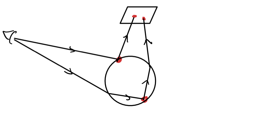
In this final project, I implement photon mapping techniques and combine it with the path tracer. The rendering process takes two passes. In the first pass, photons are shot from light sources toward glass objects only, and cached on the first non-glass surface they hit. In the second pass, rays are shot from the camera, and on each intersection, we compute its radiance by adding up NEE and caustics calculated from the photon map. Then, we do the recursive path tracing and terminate based on Russian roulette.
During this project, I rely heavily on Professor Jensen’s paper and course notes on photon mapping. Other online tutorials on photon mapping, reflection and refraction are also consulted during my implementation. All the materials I referred are provided at the end. I also want to say thanks to professor Ramamoorthi, and our TAs Kuznetsov and Shafiei. They gave me many advice throughout the project. Below, I will document my implementations in detail.
Glass BSDF
The first component of the project is a correct glass BSDF that describes how rays reflect and refract with glass surfaces. Whether to reflect or refract is determined randomly based on current Fresnel term, which is approximated by Schlick approximation:
$$
R(\theta) = R_0 + (1 - R_0) \cdot (1 - cos\theta)^5,
R_0 = \left(\frac{n_1 - n_2}{n_1 + n_2}\right)^2
$$
Here, $n_1, n_2$ are refraction indices of two materials. These terms are used in refraction calculation as well. I choose $1.5$ for the glass, and $1$ for the air. Whether the ray is shooting from air to glass, or from glass to air is handled by checking against the normal vector.
When the random number is higher than Fresnel term, rays get refracted. When the random number is lower than Fresnel term, rays get reflected. Also, special case of total inner reflections would also happen in refraction case, and is calculated accordingly. Directions of reflection and refraction are computed following mirror reflection equation and Snell’s equation for refraction. Corresponding BSDFs and PDFs are computed as:
$$
f_{TIR} = \frac{1}{\mid cos\theta_i \mid}, \ pdf_{TIR} = 1
$$
$$
f_{reflect} = \frac{R(\theta_i)}{\mid cos\theta_i \mid},
pdf_{reflect} = R(\theta_i)
$$
$$
f_{refract} = \frac{1 - R(\theta_i)}{\mid cos\theta_i \mid},
pdf_{refract} = 1 - R(\theta_i)
$$
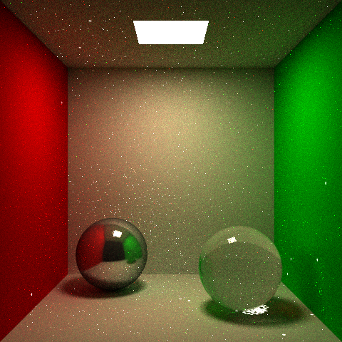
Lastly, to handle NEE correctly, I treat glass object as nontransparent, so there would be just shadows. Then, I turn off NEE for glass object. Instead, I let rays that reflect on glass object also add the kEmission term on next non-glass intersection. This would reproduce the glossy effect on glass materials accurately. Other materials are still handled by NEE, and kEmission is added only in first intersection.
Note total inner reflections are considered as reflection in above strategy as well. The highlight on bunny’s ears not only comes from upper surface reflection, but also total inner reflection from the lower surface.
| Glass Sphere without Caustics | Glass Bunny without Caustics |
|---|---|
 |
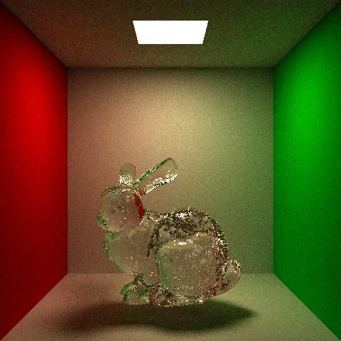 |
Photon Caching
The next step would be shooting photons, tracing photons and caching them on the surface. Shooting photons is implemented as a new OptiX ray generation device written in PhotonMapper.cu. Tracing photons is handled by adding another ray type and corresponding closeHit program defined in PhotonTracer.cu.
Hundreds of photons are generated from each square light source. Each photon’s initial position is sampled uniformly on the square light source, and direction is sampled from a cosine distribution. The initial intensity is then given by: $I_p = \frac{I_l \cdot A_l \cdot \cos\theta}{\frac{\cos\theta}{\pi}} = I_l \cdot A_l \cdot \pi$, where $I_l$ is the intensity of the light source and $A_l$ is the area of the light source.
During the photon shooting stage, the closeHit program check if it hits a glass object, and only do recursive trace if the photon hit a glass surface first. This essentially is an additional rejection sampling, and the count of actual trails is recorded in a buffer that would be divided in the intensity of the photon later.
On each intersection with glass surface, the next direction is calculated by calling BSDF sampling function for glass object. The intensity is then timed by the corresponding BSDF. Once the photon gets out of glass object and hit a diffuse surface, its position, intensity and direction are stored in a buffer holding all photons.
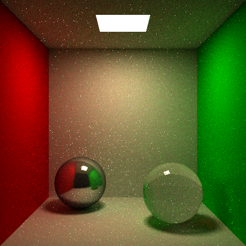
Below are some virtualizations of how photons are cached on diffuse surfaces. The integrator turn radiance to $1$ if a pixel is close enough to a photon. This is a helpful debug function I used frequently.
| Glass Sphere with Cached Photons | Glass Bunny with Cached Photons |
|---|---|
 |
Path Tracing with Photon Mapping
The last step would be path tracing and estimate caustics by photon mapping. These are implemented in PMPathTracer.cu as a new integrator, and can be used in scene file by including integrator photonmapping. The photon virtualization function I mentioned above, and the calculation of caustics from photon map are both written in this new path tracer.
Caustics are calculated based on density estimation of photons. Because of limited time and the limitation in OptiX, I stored photons in a naïve linear buffer. On each intersection, nearest photons are searched linearly, and inserted into a binary heap where distance is the priority. This would make the root element having largest distance. So, once the heap is full, we replace the root if we find a closer photon, and then sort to heap order. This binary heap was initially implemented using primitive array defined in heap.h. But, it turns out when the size get larger, the memory on GPU got messed up. Thus, the final version is implemented using a huge buffer of size $width \cdot height \cdot heapSize$. Each ray for each pixel will have their own space to maintain the heap, and would not interfere with each other.
With a working heap that can store any number of nearest photons, the caustic estimation is given by:
$$
\sum_{p=1}^N f(x, \omega_o, \omega_{i,p}) \cdot
\frac{\Delta\Phi_P(x, \omega_{i,p})}{\pi r^2}
$$
- $f(x, \omega_o, \omega_{i,p})$ is the BRDF of the intersecting position $x$ given viewing direction and photon direction.
- $\Delta \Phi_p(x, \omega_{i,p})$ is the intensity of the photon arriving at $x$ from direction $\omega_{i,p}$.
- $r$ is the largest distance of $N$ nearest photons.
Then, since further photons should have less contribution to this estimation, I adopt the cone filter which assign a weight $w_p = 1 - \frac{d_p}{r}$ for each photon. So the final estimation equation is given by:
$$
\frac{1}{\pi r^2} \cdot \sum_{p=1}^N f(x, \omega_o, \omega_{i,p}) \cdot
\Delta\Phi_P(x, \omega_{i,p}) \cdot \left(1 - \frac{d_p}{r}\right)
$$
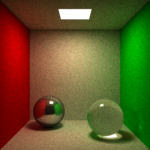
Then, we can get following results. They are rendered by the photon mapping path tracer I described above, with $64$ samples each pixel, $200$ photons from light source, and $N = 20$ in caustic estimation.
| Glass Sphere with Caustics | Glass Bunny with Caustics |
|---|---|
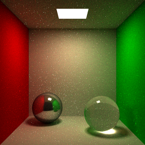 |
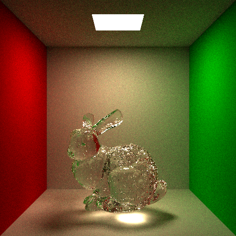 |
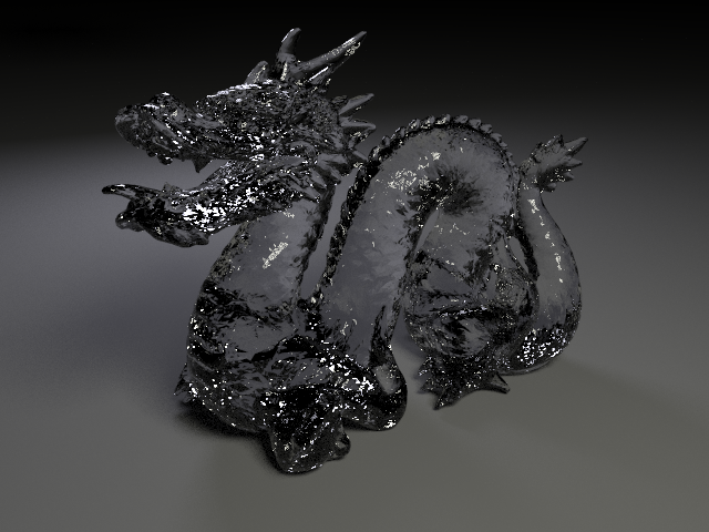
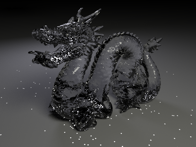
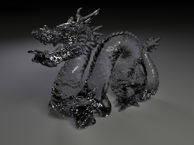
Here is a comparison of a larger scene where caustics effect is subtle. Notice how the ground around dragon’s feet are lit with caustics calculated from photon map.
| Glass Dragon without Caustics | Glass Dragon with Cached Photons | Glass Dragon with Caustics |
|---|---|---|
 |
 |
 |
Flaw
Caustics seems nice in examples I present above, but there is a flaw. Because the caustics are estimated from density distribution, they have a blur boundary and smoother looking comparing with real caustics. Maybe a better weighting function could help. Also, increasing the number of photons and adjust how many photons we collect for estimation could improve the result. But, I don’t really find a perfect set of parameters to reproduce actual details in caustics.
Here are some comparisons between path tracing results and photon mapping results:
| Path Tracing with 2048 Samples | Photon Mapping with 64 Samples |
|---|---|
 |
|
 |
|
Summary
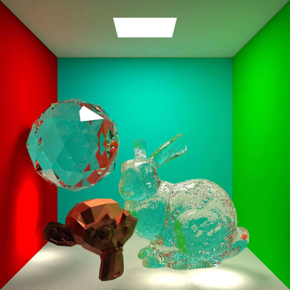
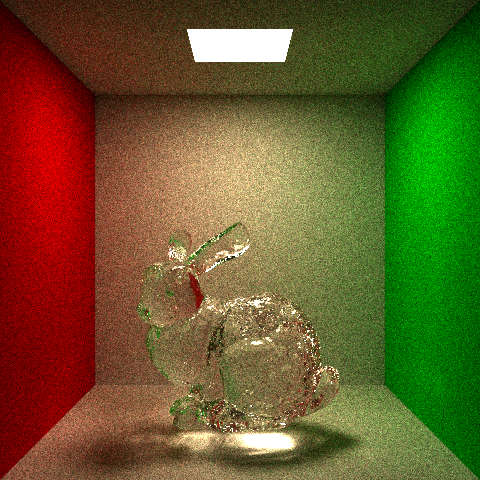
All in all, I implement a glass material and a photon mapping path tracer. I can now produce approximately correct caustics with much less number of samples thanks to the photon map. Possible improvements include a more efficient data structure storing photons, and a better estimation functions preserving details in caustics. The cover image is rendered with $2048$ samples in $1000 \times 1000$ resolution, which I think fully demonstrate the reflection, refraction and caustics effects I achieved.
Reference
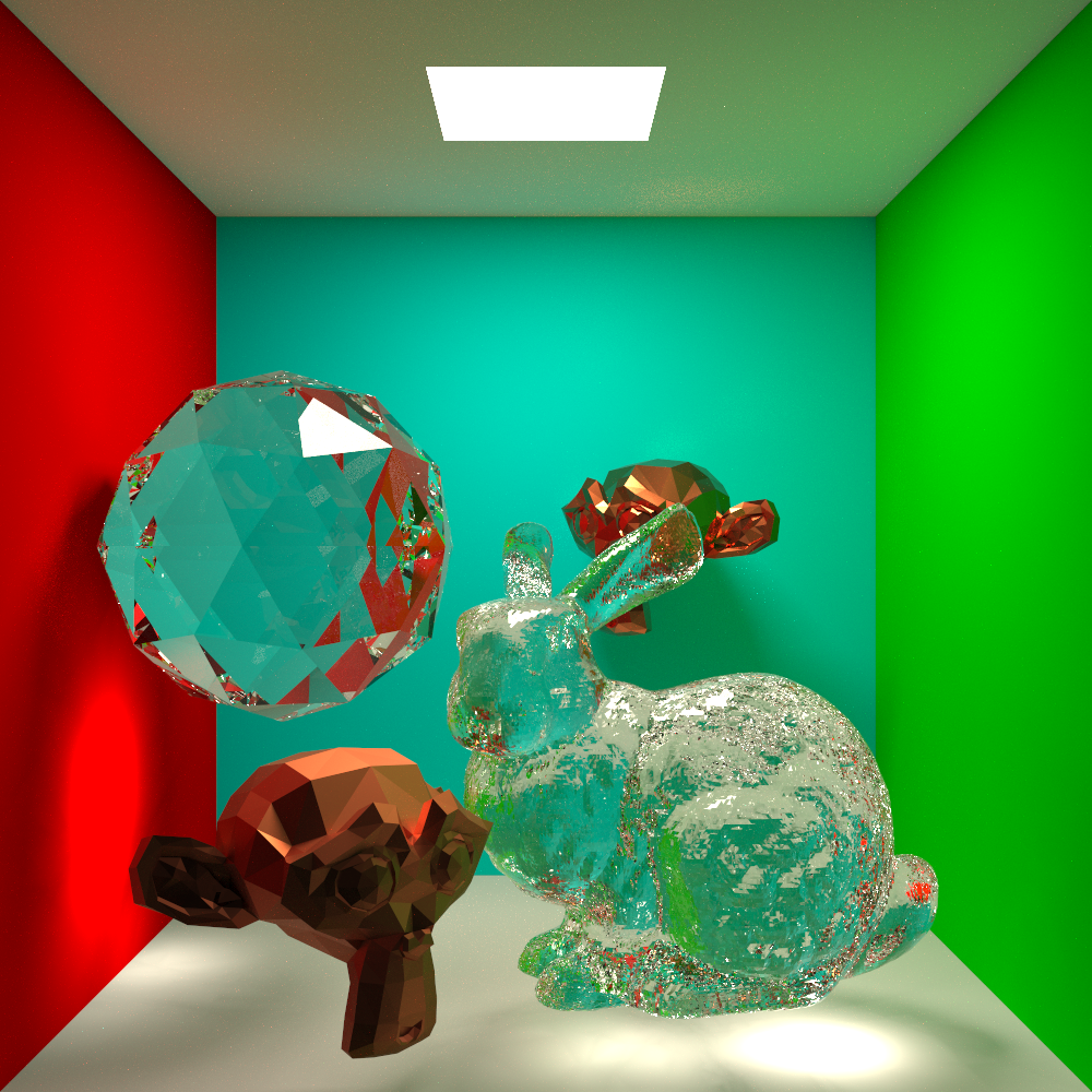
Easter Egg :-)
This is a variant of the cover image rendered with same configuration. Thanks for reading!